18 Supervised Learning Techniques
18.1 Introduction
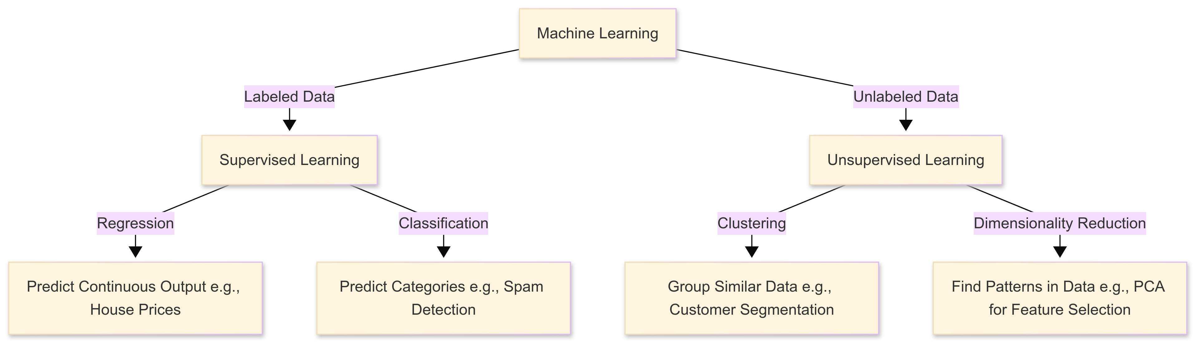
This chapter introduces the topic of machine learning, and focusses on “supervised” learning – a type of machine learning where a model is trained using labelled data. This means that, for each input, there is a corresponding known output. This allows the algorithm to ‘learn’ patterns that map inputs to correct predictions (hence the name).
Our goal in ML is to develop a model that can generalise well to unseen data, making accurate predictions based on new inputs.
Supervised learning extends traditional statistical modelling by balancing interpretability with predictive accuracy. The focus of supervised ML approaches is on optimisation; developing models that consistently deliver high-accuracy insights.
This chapter explores how machine learning goes beyond standard regression and classification in its handling of large datasets and complex relationships. We’ll examine regularised linear models (Ridge, Lasso, Elastic Net) and their role in managing multicollinearity and improving generalisation.
The chapter also covers models such as Support Vector Machines and explores decision tree ensembles, from Random Forests to powerful Gradient Boosting methods like XGBoost.
18.2 What is ‘Machine Learning’?
18.2.1 Introduction
Machine learning techniques differ from classical statistical approaches in their core objectives and assumptions. While traditional methods focus on inference, which means drawing conclusions about populations from sample data, machine learning prioritises predictive accuracy, scalability, and algorithmic optimisation.
This shift in emphasis means that advanced ML techniques often incorporate sophisticated regularisation, hyperparameter tuning, and data-driven validation methods to maximise performance on unseen data, rather than more traditional concerns around parameter estimation and significance testing.
18.2.2 What is ‘regularisation’?
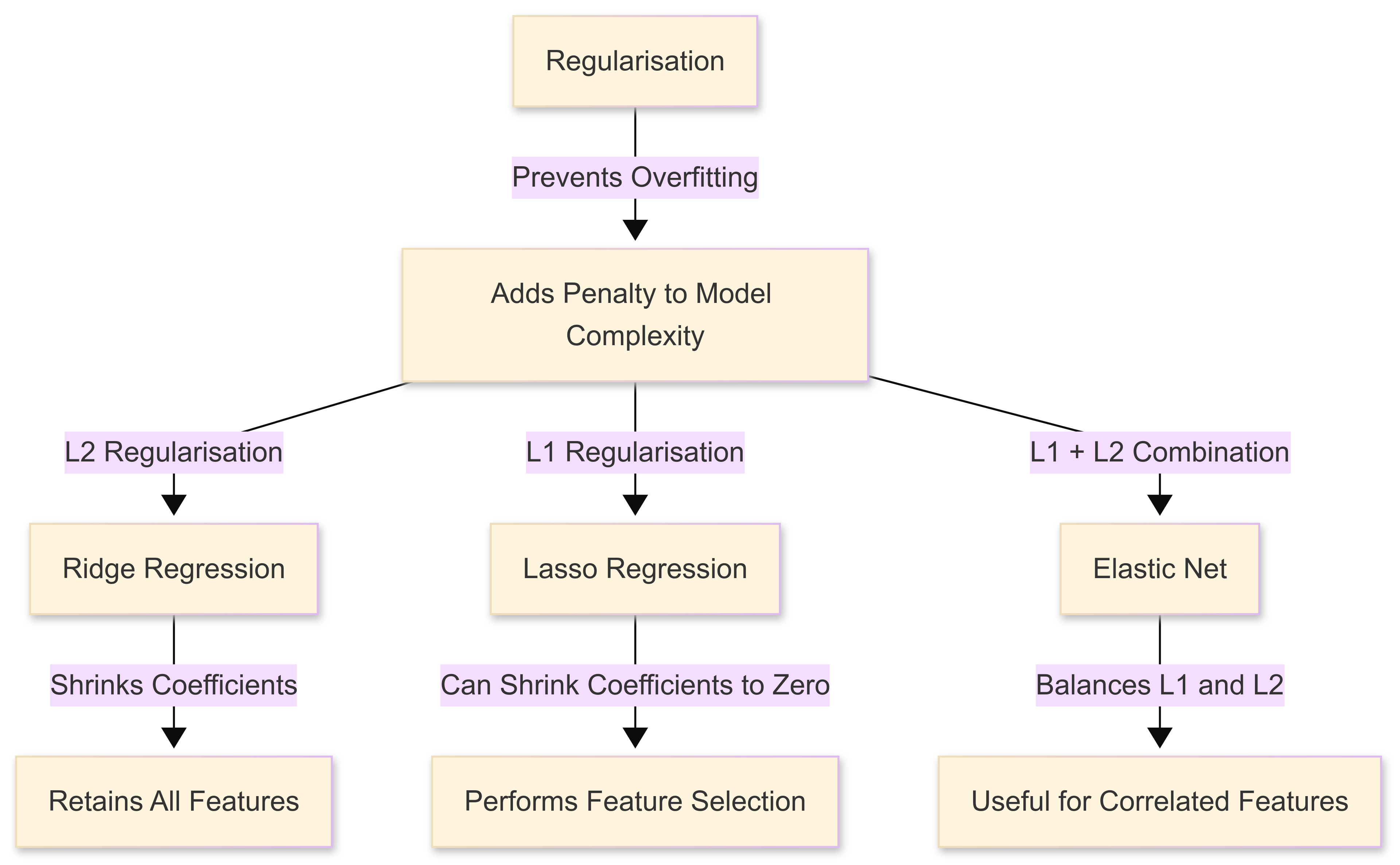
Regularisation in machine learning refers to techniques that prevent models from overfitting by adding a penalty to overly complex solutions.
Remember: ‘overfitting’ occurs when a predictive model captures noise rather than true patterns, leading to poor generalisation on unseen data.
Regularisation constrains the model’s flexibility, ensuring that it remains both interpretable and robust, particularly in high-dimensional datasets where multicollinearity can distort predictions. We’ll cover this topic in more detail later in the chapter.
18.2.3 Machine learning in sport
In sport data analytics, where prediction (e.g., anticipating player performance, match outcomes, or injury risk) can guide critical decisions, the capacity of machine learning models to adapt and improve as data evolves is especially powerful in addressing the following issues:
Issue 1: High dimensionality
Such adaptability becomes crucial when dealing with challenges characteristic of sports data. High dimensionality, for instance, arises when we incorporate numerous player attributes, training metrics, or environmental factors, often resulting in datasets with hundreds or thousands of features. In traditional approaches, excessive features in the model can lead to overfitting or unstable estimates.
Advanced ML algorithms manage this complexity using regularisation or feature selection techniques that improve generalisation of our predictive models.
Issue 2: Multicollinearity
Equally important is the problem of multicollinearity, where overlapping variables (such as correlated movement metrics or performance indicators) reduce the reliability of coefficients in classical statistical models.
Machine learning methods like Ridge or Lasso regression handle these correlations more gracefully, ensuring more stable predictions and enhanced interpretability.
Issue 3: Time-dependent characteristics
Additionally, sport data frequently exhibit time-dependent characteristics. Performance measures and physiological data collected across multiple training sessions or matches may show temporal autocorrelation. Classic statistical models often assume independence between observations, complicating the analysis of trends or patterns that unfold sequentially.
Advanced approaches, including recurrent neural networks or specialised time-series machine learning algorithms, explicitly model these dependencies, capturing the evolving nature of athlete performance or team dynamics over time.
18.3 Regularised Linear Models
18.3.1 Introduction
As noted above, one of the advantages of ML approaches is that they involve regularisation. Regularised linear models are just normal linear regression models, but with a bit of a ‘twist’, in that they include penalties to prevent overfitting.
Think of it like adding a little resistance to stop the model from getting too fixated on quirks in the training data.
Regularisation techniques help us manage the challenges of high-dimensional data. When too many performance metrics are used, models can become unstable. This can lead to overfitting, where a model learns patterns that only apply to past data but fail to generalise to new cases. Regularisation prevents this by adding penalties to large or unnecessary coefficients, simplifying the model while maintaining accuracy.
18.3.2 Key regularisation techniques: Ridge, Lasso, and Elastic Net
You’ll encounter a number of techniques that are commonly used to perform this regularisation:
Ridge regression (L2 penalty)
Ridge regression is a type of linear regression that incorporates regularisation to prevent overfitting, which occurs when a model becomes too closely tailored to the training data and struggles to perform well on new data.
It does this by adding a penalty term to the standard least squares regression equation. This penalty is proportional to the sum of the squared values of the model’s coefficients, controlled by a tuning parameter known as lambda (λ). When λ is set to zero, ridge regression is identical to ordinary least squares regression. As λ increases, the penalty grows, forcing the model to shrink the coefficients towards zero.
Unlike Lasso regression (below), which can eliminate some variables by reducing their coefficients to exactly zero, ridge regression retains all features but reduces their influence, helping to address multicollinearity (where predictor variables are highly correlated).
The main advantage of ridge regression is its ability to improve generalisation when working with datasets that contain many correlated variables or noisy data. By constraining coefficient sizes, it prevents the model from giving excessive weight to any one feature, leading to more stable predictions.
However, since it doesn’t perform feature selection (i.e., it does not eliminate variables entirely), it’s most useful when all predictors contribute some degree of useful information, even if weakly. Ridge regression is widely used in practical applications like finance, genetics, and image processing, where large, complex datasets require robust predictive modelling.
Choosing an appropriate value for λ is crucial and is typically done using cross-validation, where different values are tested to find the one that offers the best balance between bias and variance.
Lasso regression (L1 penalty)
Lasso regression (Least Absolute Shrinkage and Selection Operator) is a form of linear regression that, like ridge regression, incorporates regularisation to improve a model’s generalisation and prevent overfitting.
However, instead of penalising the sum of squared coefficients as in ridge regression, lasso applies a penalty based on the absolute values of the coefficients. This L1 regularisation technique forces some coefficients to shrink exactly to zero when the penalty is sufficiently strong.
The extent of this shrinkage is controlled by something called the lambda (λ) parameter:
A small λ results in minimal regularisation, making lasso behave like ordinary least squares regression;
A larger λ increases the penalty, driving weaker predictors to zero and effectively performing feature selection.
The key advantage of lasso regression is its ability to simplify models by automatically selecting the most relevant features while eliminating those that contribute little to the prediction. This makes it particularly useful when dealing with high-dimensional datasets where many predictor variables may be irrelevant or redundant. By reducing the complexity of the model, lasso can improve interpretability and efficiency.
However, when our predictor variables are highly correlated, lasso may arbitrarily select one while disregarding others, which can be a limitation. As with ridge regression, choosing the optimal λ is crucial, and is typically determined through cross-validation to find the best trade-off between sparsity and predictive accuracy.
Elastic Net
Elastic Net regression is a hybrid approach that combines the strengths of both ridge and lasso regression. It applies L1 (lasso) and L2 (ridge) regularisation simultaneously, balancing feature selection and coefficient shrinkage.
The model includes two tuning parameters: lambda (λ), which controls the overall strength of regularization, and alpha (α), which determines the mix between L1 and L2 penalties. When α = 1, the model behaves like pure lasso regression, emphasizing feature selection by shrinking some coefficients to zero. When α = 0, it acts as ridge regression, shrinking coefficients without eliminating any predictors. By adjusting α, Elastic Net allows for a flexible approach that can handle different types of data structures more effectively than lasso or ridge alone.
The main advantage of Elastic Net is its ability to handle situations where predictors are highly correlated, a challenge that can cause lasso to arbitrarily select one variable while ignoring others. By incorporating an L2 component, Elastic Net distributes coefficient weight more evenly among correlated variables, making it particularly useful in cases where multiple predictors share similar importance.
This technique is widely used in fields where datasets contain a large number of interdependent variables. Like ridge and lasso regression, Elastic Net requires careful selection of its tuning parameters, typically done through cross-validation, to find the best balance between sparsity, stability, and predictive performance.
18.3.3 Generalised Linear Models
Introduction
Machine learning provides a wide range of tools for predictive modelling, and one particularly powerful class of models is the Generalised Linear Model (GLM).
GLMs extend standard linear regression to handle different types of response variables, making them highly flexible for real-world applications where our data isn’t always continuous or normally distributed. This adaptability is particularly useful in sport analytics, where our data can take various forms (e.g., binary outcomes, counts, or skewed continuous values).
Unlike ordinary linear regression, which assumes a continuous response variable with normally distributed errors, GLMs introduce a link function that transforms the relationship between the predictors and the response variable. This allows them to model a broader range of data structures, making them more effective for different types of sports-related predictions.
We’ll briefly review some of the most common GLMs used currently.
Logistic Regression (Binary Outcomes)
Logistic regression, a type of GLM, is ideal for modelling binary classifications, such as predicting whether a player will sustain an injury (injured vs. not injured) or whether a team will win a match (win vs. lose).
By using the logit link function, it estimates the probability of an event occurring, making it a fundamental tool in risk assessment and player performance evaluation.
Poisson Regression (Count-Based Data)
When dealing with count data, such as the number of goals scored per match, tackles made, or fouls committed, Poisson regression is a good choice. It assumes that the dependent variable follows a Poisson distribution; a probability distribution used to model the number of times an event occurs in a fixed interval of time or space, assuming the events happen independently and at a constant average rate.
This makes it useful for situations where the outcomes represent discrete events occurring within a fixed period or space. In sport, Poisson models are appropriate when forecasting match scores, analysing team performance, or estimating player contributions in specific statistical categories.
Gamma Regression (Skewed Continuous Data)
In some cases, response variables are continuous but positively skewed, meaning they cannot be accurately modelled with standard linear regression. A Gamma GLM is well-suited for this scenario, and could usefully be applied to sports metrics such as energy expenditure, playing time, or recovery duration.
Basically, it helps analyse situations where the variance increases with the magnitude of the response, making it useful in contexts where data follows an exponential-like distribution.
18.3.4 Hyperparameter tuning and model validation
To make these models reliable, we must tune hyperparameters. Hyperparameters are the settings that control how a model learns, and are a key feature of machine learning approaches.
Methods like k-fold cross-validation test models on different sections of data to check consistency. Bayesian optimisation and grid/random search fine-tune regularisation parameters (like alpha for Lasso or lambda for Ridge) to improve generalisation.
In practice, these techniques (which are beyond the scope of this module) help refine models, ensuring they remain both accurate and interpretable.
18.4 Support Vector Machines and Kernel Methods
18.4.1 Introduction
While regularised linear models such as ridge, lasso, and elastic net improve the stability and generalisability of linear regression, they still rely on the assumption that relationships between predictors and the target variable are linear.
However, many real-world problems involve complex, non-linear relationships that linear models struggle to capture effectively. This is where Support Vector Machines (SVMs) come in.
By introducing the concept of decision boundaries and leveraging kernel functions, SVMs can model both linear and non-linear relationships, making them a powerful alternative when ‘simple’ linear methods fall short.
18.4.2 Kernel Functions
Support Vector Machines (SVMs) rely on kernel functions to map complex data into higher-dimensional feature spaces, enabling the separation of data points that are not linearly separable in their original space.
The polynomial kernel, for instance, transforms input features by incorporating polynomial terms of a chosen degree \(d\), effectively capturing non-linear interactions between variables such as a player’s endurance, technique, and environmental conditions (e.g., pitch surface).
The radial basis function (RBF) kernel is another powerful alternative that relies on a Gaussian-like transformation to measure similarity between data points, thereby adapting more dynamically to highly intricate, non-linear data structures commonly observed in sport analytics; imagine large datasets of players with intersecting skill sets or movement patterns that require nuanced discrimination.
Beyond these widely used kernels, ‘custom’ kernels can be devised for specialised domains, such as incorporating domain-specific distance metrics or prior knowledge about time-series correlations in sports data, thereby offering a targeted approach for complex predictive tasks.
18.4.3 More on Kernel Functions
Mathematically, the kernel trick hinges on defining an inner product in a (potentially) infinite-dimensional space without explicitly computing the coordinate transformation.
For an RBF (Radial Basis Function) kernel of the form
\[ k(\mathbf{x}, \mathbf{x}') = \exp\left(-\gamma \|\mathbf{x} - \mathbf{x}'\|^2\right) \]
the hyperparameter \(\gamma\) controls the “smoothness” of the decision boundary. Larger values of \(\gamma\) allow the model to capture more complex patterns, but they also increase the risk of overfitting by making the model too sensitive to individual data points.
For polynomial kernels of the form
\[ k(\mathbf{x}, \mathbf{x}') = (\mathbf{x}^\top \mathbf{x}' + c)^d \]
the degree \(d\) and constant \(c\) greatly influence model flexibility. Higher values of \(d\) allow the model to fit more complex relationships, but they can also lead to overfitting if not properly regularised.
Hyperparameter optimisation thus becomes crucial: analysts often employ grid search or Bayesian optimisation in tandem with cross-validation to systematically explore kernel-specific parameters alongside \(c\), the penalty for misclassifications.
Techniques like nested cross-validation can help mitigate the risk of overfitting and provide more reliable estimates of generalisation performance.
18.4.4 SVMs in Sport
In a sporting context, SVMs with advanced kernels are exceptionally useful for tasks ranging from player classification (e.g., distinguishing forwards, midfielders, defenders based on multi-dimensional performance metrics) to tactical decision-making (e.g., predicting successful passing lanes or strategies under varying match conditions).
For instance, an RBF-kernel SVM might classify possession sequences according to attacking or defensive effectiveness, drawing upon detailed spatiotemporal features (e.g., player positions, distances, and velocities) across multiple time points.
Meanwhile, a custom kernel might embed domain-specific insights about pitch geometry or physiological markers, allowing us to highlight the specific interactions most relevant to performance.
By tuning kernel parameters methodically and validating against metrics such as precision, recall, or AUC, we can achieve robust, generalisable results that inform decision-making at both the coaching and managerial levels.
18.5 Advanced Decision Trees and Extensions
18.5.1 Introduction
Support Vector Machines are particularly effective for classification tasks, especially when working with high-dimensional data. However, they can become computationally expensive as dataset size grows and may not always be the most interpretable model.
In contrast, advanced decision tree-based models, such as Random Forests and Gradient Boosting Machines, offer a flexible and scalable approach to both classification and regression.
These models build upon the simplicity of traditional decision trees by using ensembles of multiple trees to improve predictive accuracy and robustness, often outperforming SVMs in large, complex datasets.
18.5.2 CART
CART (Classification and Regression Trees) provide a robust framework for decision tree models by recursively partitioning the feature space into homogenous subsets, ultimately producing rule-based segments that are simple to interpret.
While CART’s transparency and ease of implementation make it appealing, it can be prone to overfitting unless carefully regularised. In a sport analytics context, for example, predicting whether a basketball player will be sidelined by injury—CART alone can give valuable initial insights but might not capture the full complexity of multi-faceted training loads, physiological markers, and historical data.
Building on this concept, Random Forests improve predictive performance and reduce overfitting by aggregating multiple decision trees trained on bootstrapped samples with randomised feature subsets. This “bagging” approach is especially useful in high-dimensional sports datasets. For instance, an analyst exploring numerous performance, biometric, and psychological metrics for player valuation could rely on Random Forests to handle multicollinearity and complex interactions.
We’ll cover bagging in more detail in the next chapter.
Hyperparameter tuning, such as selecting the optimal number of trees (n_estimators) and max_features, can drastically improve performance. Gradient Boosting, on the other hand, grows trees sequentially, iteratively refining errors from previous trees.
It’s more sensitive to parameter choices like learning rate and depth but can uncover subtle relationships hidden in large feature sets, making it particularly effective for performance forecasting, such as predicting an athlete’s season-long progression based on training workloads and early-season form.
18.5.3 XGBoost
XGBoost is one of the most powerful and widely used machine learning algorithms, particularly in predictive modelling tasks where speed and accuracy are critical. It belongs to a class of models known as gradient boosting, which builds multiple decision trees in sequence.
Unlike traditional decision trees, where each tree is built independently, boosting methods like XGBoost train each new tree to correct the mistakes of the previous ones. This step-by-step learning process allows the model to make better predictions with each iteration. The result is a strong, high-performance model that often outperforms simpler approaches like linear regression or standalone decision trees.
We’ll cover boosting in more detail in the next chapter.
A major advantage of XGBoost is its ability to handle both structured and unstructured data while effectively managing missing values. Unlike some other machine learning methods, it does not require all input data to be perfectly complete. Instead, it can intelligently determine the best way to handle missing values, making it highly practical for real-world datasets where gaps and inconsistencies are common. Another reason for its success is its use of second-order gradient information, which refines predictions more effectively than traditional boosting methods.
Additionally, XGBoost includes advanced regularisation techniques, such as lambda and alpha parameters, which (as we know) help prevent overfitting by controlling the complexity of the model. These features make it particularly suited for working with large, complex datasets.
One key advantage of XGBoost is its interpretability. Unlike some complex machine learning models, which act as black boxes, XGBoost provides tools that help us understand how it reaches its predictions.
Feature importance scores indicate which variables have the greatest influence on the model’s decisions, while SHAP (Shapley Additive Explanations) values provide insight into the contribution of each feature to individual predictions.
In sport analytics, for example, these tools could be invaluable for answering questions such as which factors contribute most to a player’s injury risk, or which performance metrics best predict future success.
18.6 Model Evaluation and Selection
18.6.1 Introduction
Advanced decision tree models can be highly effective, but their performance depends on careful tuning of hyperparameters such as tree depth, learning rate, and the number of trees in an ensemble.
This highlights the broader challenge of model evaluation and selection—choosing the most appropriate model for a given problem based on performance metrics and validation techniques.
Comparing models using approaches such as cross-validation, precision-recall analysis, and ROC curves ensures that the final choice balances predictive power, interpretability, and computational efficiency.
18.6.2 Nested cross-validation
Nested cross-validation addresses two key challenges simultaneously: selecting optimal hyperparameters and estimating unbiased out-of-sample performance.
In the “outer loop,” the data is split into training and test folds to measure final performance, while in the “inner loop,” various hyperparameter configurations are tested on cross-validated subsets of the training fold.
This approach reduces the risk of overly optimistic performance estimates.
18.6.3 Bayesian optimisation
Bayesian optimisation further refines this process by systematically searching the hyperparameter space using a probabilistic model. Rather than sampling hyperparameter configurations randomly or exhaustively (as in grid search), Bayesian optimisation uses prior evaluations to update beliefs about promising parameter regions. It’s effectively learning where to sample next to maximise improvements.
This is particularly useful when dealing with computationally expensive models, such as deep neural networks or large ensemble methods. By iteratively ‘honing in’ on the best hyperparameter settings, we can uncover nuanced interactions between parameters that standard search strategies might miss, leading to consistently stronger model performance.
18.6.4 ROC and AUC
Finally, Receiver Operating Characteristic (ROC) curves and the related Area Under the Curve (AUC) metric provide robust ways to compare classification performance across models that may have different score thresholds or class distributions.
For example, when assessing whether a model can reliably predict whether an athlete will sustain a hamstring injury, the AUC offers a threshold-independent assessment of sensitivity and specificity.
In practice, we often combine AUC with domain-specific metrics such as cost-sensitive measures for misclassifications, especially in high-stakes sporting contexts where a misjudged injury risk or scouting decision can be extremely costly!